Reading Jia-Wei Hong and H. T. Kung, I/O Complexity: The Red-Blue Pebble Game, STOC 1981, pp. 326–333. Original paper
Imagine an infinitely fast processor whose workbench holds only ten numbers. To process a million numbers, it still has to bring them in from storage. Intermediate results that do not fit must travel out, and perhaps return later.
This 1981 paper studies exactly that limitation. A simple game turns the movement caused by finite fast memory into a mathematical problem with provable bounds. Later work on communication-optimal matrix multiplication and attention I/O follows the same line of thought.
From an expression to a computation graph
Consider
The dependencies form a DAG:
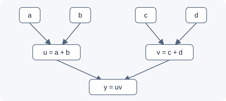
A vertex represents a value or the operation producing it; an edge represents a dependency. We cannot compute $y$ without $u,v$.
The graph specifies which computations must happen, but neither their execution order nor which intermediate values remain in memory. Different schedules can evaluate the same graph with different amounts of movement.
Two pebble colors, two storage levels
A red pebble means a value is in fast memory; a blue pebble means it is in slow memory. A vertex may carry both colors, representing a copy at each level.
There are at most $S$ red pebbles, while slow memory is unbounded. Inputs begin in slow memory, and final outputs must also be saved there.
| Operation | Game rule | Computer interpretation | Counts as I/O? |
|---|---|---|---|
| Load | Place a red pebble on a vertex carrying a blue pebble | Read from slow to fast memory | Yes |
| Store | Place a blue pebble on a vertex carrying a red pebble | Write from fast to slow memory | Yes |
| Compute | Place a red pebble on a result only when all immediate predecessors carry red pebbles | Execute an operation with its inputs ready | No |
| Delete | Remove a pebble | Free a storage position | No |
The goal is to finish the outputs while minimizing the total number of loads and stores:
We use $L$ for I/O count to avoid confusion with attention’s query matrix $Q$; the original paper uses $Q$.
One pebble represents one word. Converting traffic to bytes requires specifying the word width.
Playing the game by hand
Return to the expression above with $S=4$. Load $a,b$, compute $u$, then remove $a,b$. Load $c,d$, compute $v$, then remove $c,d$. Compute $y$ and finally store it.
Each of the four inputs is read once, and the output is written once: five I/O operations. At most four values coexist, namely $u,c,d,v$.
With less capacity, we may need to spill $u$ to slow memory and reload it later, adding one store and one load. Another possibility is to discard $u$, then reload $a,b$ and recompute it when needed.
The original game permits recomputation: its computation rule does not require each vertex to be evaluated only once. This allows a trade between extra arithmetic and less storage. Some later models forbid recomputation, so a lower bound must be read with its model version in mind.
Why not search every possible play?
Small graphs can be enumerated, but the number of legal schedules grows rapidly. Rather than finding the best play for every DAG, Hong and Kung ask a static question: how many subcomputations with bounded boundaries are needed to partition this graph?
If each subcomputation can perform only limited work, a large problem needs many phases. More phases force more movement.
This is a proof technique. It establishes costs no legal execution can avoid, but does not automatically produce an optimal program.
Where the factor 2S comes from
Cut an execution into consecutive phases, each complete phase containing exactly $S$ I/O operations. The last phase may contain fewer.
At phase entry, fast memory contains at most $S$ values, and the phase can load at most $S$ more. Its supporting boundary information is therefore at most $2S$. At phase exit, at most $S$ values remain in fast memory, and at most $S$ can have been stored, so the output boundary is also at most $2S$.
This induces a $2S$-partition. The original definition requires four properties: disjoint parts covering the whole graph, a small dominator set for each part, a small minimum set for each part, and no cyclic dependencies between parts.
A dominator set is a collection of unavoidable entrances: every path from an input to a vertex in the part passes through it. It need not coincide with array elements directly read by source code.
The minimum set consists of vertices in a part with no successor remaining in that part. These are exits of the internal computation; minimum does not refer to numerical values.
This phase argument explains $2S$, but the rigorous construction must handle recomputed vertices. Occurrences during execution cannot simply be declared disjoint parts of a static graph.
The central lemma
Let $P(G,2S)$ be the smallest number of parts among valid $2S$-partitions. Lemma 3.1 states
Why subtract one? The final phase need not consume all $S$ I/O operations.
Suppose the graph contains $W$ computation vertices being counted, and each legal part contains at most $U(2S)$. Then
Substituting gives
This is a practical proof template: bound the work supported by a finite boundary, then divide total work by that bound. The difficulty usually lies in bounding $U(S)$, rather than enumerating schedules.
Matrix multiplication: why n³/√S transfers are necessary
Classical $n\times n$ matrix multiplication requires $n^3$ scalar multiplications:
A subset of these multiplications can be represented as a set of triples $T\subseteq\lbrace(i,j,k)\rbrace$. Its projections onto the three coordinate planes correspond to the entries of $A$, $B$, and the partial sums of $C$ that it uses.
A modern geometric explanation uses a discrete Loomis–Whitney-type inequality:
If each projection contains only $O(S)$ elements, then
A subcomputation constrained by that memory boundary thus supports only $O(S^{3/2})$ useful multiplications. At least
subcomputations are required. Multiplying by the $S$-operation I/O budget per phase yields
The projection inequality explains the exponent; it is not a claim that the original paper uses this proof language. Section 6 derives the ordinary matrix multiplication result through independent computations and counting. A formal proof cannot equate the number of values currently in fast memory with an entire phase’s boundary.
The rectangular version is
under the corresponding computation and dimension assumptions. If inputs start in slow memory and outputs must be written back, compulsory I/O also matters. A common asymptotic expression is
with the memory and rectangular-dimension regime checked explicitly. Even a large memory must read inputs and write outputs.
Can the lower bound be attained?
Use square tiles of side length $b=\Theta(\sqrt S)$. Two input tiles and one output tile require $\Theta(b^2)$ fast-memory space, and each local product completes $\Theta(b^3)$ multiply-adds.
There are approximately $(n/b)^3$ tile products, each requiring $O(b^2)$ traffic, giving
The upper and lower bounds match in order, so the square-root relation reflects a real limitation. Quadrupling memory roughly halves the leading communication term; doubling it improves that term by only about $\sqrt2$.
Why FFT has log S instead
The FFT graph has $\Theta(n\log n)$ computation vertices. The paper shows that a part with boundary size $O(S)$ contains at most $O(S\log S)$ vertices. Thus
In the usual regime $2\le S\le n$, a suitable decomposition achieves the same order. Intuitively, a local FFT of size $S$ can complete about $\log S$ layers while resident in fast memory. The whole graph has about $\log n$ layers and therefore needs repeated movement across the boundary.
Matrix multiplication and FFT have different reuse structures, so increased capacity benefits them differently. One rule for how much doubling memory improves performance cannot describe every algorithm.
Other graphs in the paper
The paper also analyzes information propagation speed, odd-even transposition sorting networks, snake-like meshes, and graph products.
For example, a local region of scale $r$ in a $d$-dimensional directed mesh has roughly $r^d$ vertices but needs roughly $r^{d-1}$ boundary information. If that boundary is limited by $S$, then
For the corresponding graph with $m^d$ vertices, this relationship leads to a related I/O lower bound of
The original paper establishes this using a graph-product theorem for dominators. The volume-and-boundary argument above provides intuition. This discussion assumes $d\gt 1$, as required by the exponents.
A common theme emerges: the geometry of dependencies determines how much work a small workbench can sustain.
From I/O lower bounds to hardware performance limits
The following applies the paper to modern performance estimation. If at least $L_{\min}$ words must move, each occupies $w$ bytes, and the relevant boundary has bandwidth ceiling $\beta$, then
If the specified algorithm also needs at least $F_{\min}$ FLOPs and hardware peak compute at the matching precision is $P$, then
This connects a movement lower bound to Roofline. An optimistic time lower bound can be derived without measuring an existing kernel’s actual traffic.
For example, if a bound with proven numerical constants requires at least 8 GB of movement and the bandwidth ceiling is 400 GB/s, runtime is at least 20 ms. If the task generates $R$ tokens, the corresponding throughput upper bound is $R/0.020$ tokens per second.
An $\Omega(\cdot)$ expression without usable constants cannot be treated as an exact byte count. The compute peak must also match the operation type and precision.
What exactly is optimal?
The most important qualification is that the red-blue pebble game starts from a given computation graph.
Within that graph, we can change execution order, tiling, residency, and even allow recomputation. A different mathematical algorithm may have an entirely different graph. A lower bound for ordinary matrix multiplication does not automatically rule out Strassen. A bound for one attention graph does not automatically constrain approximate attention.
We can say that every legal schedule of this DAG obeys the bound. A claim about every algorithm solving the underlying problem requires a specified algorithm class or stronger algebraic, communication, or information-theoretic arguments.
The game also leaves many hardware constraints outside the model: SIMD width, Tensor Core instruction shapes, parallelism, synchronization, cache-line granularity, and multiple memory levels. It captures movement limits rather than simulating a complete machine.
Using the result in a Bound Estimator
First fix the model and workload, then specify permitted transformations: operator fusion, recomputation, approximation, quantization, and the memory level where inputs and KV state already reside.
For that scope, establish a DAG or algorithm class, prove necessary computation and communication, and map them to hardware resources. If operators can be fused, their isolated writeback lower bounds cannot simply be added: intermediate data may never leave fast memory.
The resulting theoretical limit then has a precise meaning. The value of the red-blue pebble game is to make the claim that every kernel must move this much data something we can inspect, prove, and challenge by examining its assumptions.
Where to read in the original
- Printed page 327, Section 2: game rules and the two-level storage interpretation.
- Printed pages 328–329, Section 3: partitions, Theorem 3.1, and the central Lemma 3.1.
- Section 4: the FFT lower bound.
- Sections 5–6: information propagation and independent computations; Corollary 6.2 gives the ordinary rectangular matrix multiplication lower bound.
- Sections 7–8: graph products, the decomposability factor, and the conclusion.
PDF page 1 corresponds to printed page 326. This is an original exposition; the projection inequality, worked example, and modern hardware conversions are explanations rather than a sentence-by-sentence translation of the paper.