CS231n Lecture Note V: Convolution Neural Networks Basics

When images get really large, we would have too many neurons to train in a regular neural network. The full connectivity is wasteful and the huge number of parameters would quickly lead to overfitting. What’s more, regular neural networks ignore the spatial structures of the image, missing out on some important information.

As a result, a new type of neural network, the Convolutional Neural Network (CNN) was developed.

Feature Extraction

Extract features from raw pixels to feed the model with more information.

Examples include Color Histogram and Histogram of Oriented Gradients. Hand-engineered features (e.g., HOG, SIFT) are largely obsolete in modern deep learning pipelines.

Stack them all together.

Traditional feature extraction is manually designed and fixed; CNNs learn hierarchical feature representations end-to-end.

Data and compute can solve problems better than human designers?

Linear Classification Intuition

Matrix multiplication involves vector dot products. Dot products measure how strongly an input aligns with learned feature directions, which act like soft, continuous templates.

Architecture

ConvNets use convolution and pooling operators to extract features while respecting 2D image structures.

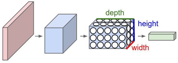
The input remains a 3D tensor (e.g. 32x32x3), preserving spatial structures.

The layers of a ConvNet have neurons arranged in 3 dimensions: width, height, depth.

The neurons in a layer will only be connected to a small region of the layer before it.

We use three main types of layers to build ConvNet architectures: Convolutional Layer, Pooling Layer, and Fully-Connected Layer (exactly as seen in regular Neural Networks).

A simple ConvNet could have the architecture [INPUT - CONV - RELU - POOL - FC].

• CONV layer will compute the output of neurons that are connected to local regions in the input, each computing a dot product between their weights and a small region they are connected to in the input volume.
• POOL layer will perform a downsampling operation along the spatial dimensions (width, height).

ConvNets transform the original image layer by layer from the original pixel values to the final class scores.

The parameters in the CONV/FC layers will be trained with gradient descent.

Convolutional Layers

A convolutional layer performs a linear operation on the input using a set of learnable filters (also called kernels). Although commonly referred to as “convolution,” most deep learning libraries actually implement cross-correlation; the distinction is usually not important in practice.

The CONV layer’s parameters consist of a set of learnable filters. Each filter is spatially small but spans the full depth of the input.

Each filter typically has a single scalar bias, shared across all spatial positions in its activation map.

During the forward pass, each filter slides across the input volume. At every spatial location, the layer computes a dot product between the filter weights and the corresponding local region of the input, then adds a bias term. This produces a 2D activation map (feature map) for that filter.

A convolutional layer contains multiple filters. Each filter produces its own activation map, and these maps are stacked along the depth (channel) dimension to form the output volume. As a result, the number of filters determines the number of output channels.

Filters are initialized differently to break the symmetry.

For convolution with size $K$, each element in the output depend on a $K \times K$ receptive field. When you stack convolutional layers, the effective receptive field grows. Each deeper layer aggregates information from a larger region of the original input.

Apart from 2D conv, we also have 1D conv and 3D conv etc.

Zero Padding

Without zero-padding, feature maps may shrink with each layer. So we add padding around the input before sliding the filter.

With the input size $W \times W$, filter size $K \times K$, and padding size $P$, we get an output of size $W - K + 2 \times P$.

A common setting is to set $P$ as $\frac{K-1}{2}$, having the output of the same size of the input.

Stride

To increase effective receptive fields more quickly, we can skip some using strides.

With the input size $W \times W$, filter size $K \times K$, stride $S$, and padding size $P$, we get an output of size $\frac{W - K + 2 \times P}{2} + 1$.

In this way, we are downsampling the image and the receptive field grows exponentially.

Pooling

Pooling layers downsample a feature map by summarizing local neighborhoods.

In max pooling, a small window, such as $2 \times 2$, slides across the input and outputs the largest value in each window. This keeps the strongest local activation and reduces spatial resolution.

In average pooling, the layer outputs the mean value in each window instead of the maximum.

Translation Equivariance

CNNs use shared filters so the same local features can be detected at different positions in an image, while preserving information about where those features occur. This is called translation equivariance.