CS188 Search Lecture Notes I

Here are the lecture notes for UC Berkeley CS188 Lecture 1 and 2.

Agents

The central problem of AI is to create a rational agent. A rational agent is an entity that has goals or preferences and tries to perform a series of actions that yield the best/optimal expected outcome given these goals.

The agent exists in an environment. Together, the agent and the environment constitute the world.

Types of Agents

A reflex agent selects its action based on only the current state of the world.

A planning agent maintains a model of the world and uses this model to simulate performing various actions.

Sometimes agents fail due to wrong world models.

Task Environment

The PEAS (Performance Measure, Environment, Actuators, Sensors) description is used for defining the task environment.

The performance measure describes what utility the agent tries to increase.

The environment summarizes where the agent acts and what affects the agent.

The actuators and the sensors are the methods with which the agent acts on the environment and receives information from it.

Types of Environment

We can characterize the types of environments in the following ways:

• partially observable environments
• fully observable environments
• Stochastic environments (uncertainty in the transition model)
• deterministic environments
• multi-agent environments
• static environments
• dynamic environments
• environments with known physics
• environments with unknown physics

State Space and Search Problems

A search problem consists of the following elements:

• A state space - The set of all possible states that are possible in your given world
• A set of actions available in each state
• A transition model - Outputs the next state when a specific action is taken at current state
• An action cost - Incurred when moving from one state to another after applying an action
• A start state - The state in which an agent exists initially
• A goal test - A function that takes a state as input, and determines whether it is a goal state

A search problem is solved by first considering the start state, then exploring the state space using the action and transition and cost methods, iteratively computing children of various states until we arrive at a goal state.

A world state contains all information about a given state, whereas a search state contains only the information about the world that’s necessary for planning.

State Space Graphs and Search Trees

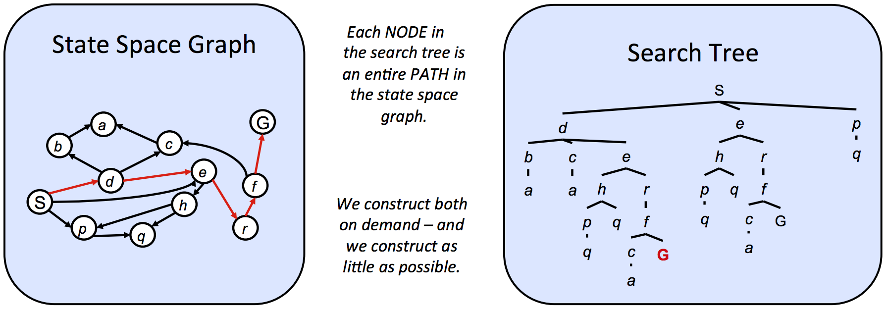
A state space graph is constructed with states representing nodes, with directed edges existing from a state to its children. These edges represent actions, and any associated weights represent the cost of performing the corresponding action.

They can be noticeably large, but they represent states well. (All states occur only once)

Search trees encode the entire path (or plan) from the start state to the given state in the state space graph.

Since there often exist multiple ways to get from one state to another, states tend to show up multiple times in search trees.

Since these structures can be too large for computers, we can choose to store only states we’re immediately working with, and compute new ones on-demand.

Uninformed Search

The standard protocol for finding a plan from the start state to the goals is to maintain an outer frontier and continually expanding the frontier by replacing a node with its children.

Most implementations of such algorithms will encode information about the parent node, distance to node, and the state inside the node object. This procedure is known as tree search.

function TREE-SEARCH(problem, frontier) return a solution or failure
    frontier ← INSERT(MAKE-NODE(INITIAL-STATE[problem]), frontier)
    while not IS-EMPTY(frontier) do
        node ← POP(frontier)
        if problem.IS-GOAL(node.STATE) then return node
        for each child-node in EXPAND(problem, node) do
            add child-node to frontier
    return failure

The EXPAND function appearing in the pseudocode returns all the possible nodes that can be reached from a given node by considering all available actions.

When we have no knowledge of the location of goal states in our search tree, we are forced to do uninformed search.

• The completeness of each search strategy - if there exists a solution to the search problem, is the strategy guaranteed to find it given infinite computational resources?
• The optimality of each search strategy - is the strategy guaranteed to find the lowest cost path to a goal state?
• The **branching factor ** - The increase in the number of nodes on the frontier each time a frontier node is dequeued and replaced with its children is . At depth k in the search tree, there exists nodes.
• The maximum depth m.
• The depth of the shallowest solution s.

Depth-First Search

Depth-First Search (DFS) always selects the deepest frontier node.

The frontier is represented by a stack.

Depth-first search is not complete. If there exist cycles in the state space graph, this inevitably means that the corresponding search tree will be infinite in depth.

Depth-first search is not optimal.

Breadth-Frist Search

Breadth-first search (BFS) always selects the shallowest frontier node.

The frontier is represented by a queue.

If a solution exists, then the depth of the shallowest node s must be finite, so BFS must eventually search this depth. Hence, it’s complete.

BFS is generally not optimal.

Iterative Deepening

Iterative Deepening (ID) is basically BFS implemented with DFS. It repeatedly executes depth-first search with an increasing depth limit.

The frontier is represented by a stack.

Iterative deepening is complete. Because it exhaustively searches each depth level before increasing the limit, it avoids the infinite loops of DFS and will find a solution if one exists at a finite depth.

ID is generally not optimal.

If the cost is uniform, ID and BFS will be optimal.

Uniform Cost Search

Uniform cost search (UCS) always selects the lowest cost frontier node.

The frontier is represented by a priority queue.

Uniform cost search is complete and optimal.

The three strategies outlined above are fundamentally the same - differing only in expansion strategy